All UCL Maths Year 1 Modules Ranked
I’ve just completed my first year at UCL studying Mathematics, and am quite pleased to be averaging a 91% :D
I thought it’d be nice to reflect a bit on the modules, so I’ll be going through each module one by one, and putting them into a tier, and hopefully giving some useful advice to those studying these modules.
Also, when I get the occasional question of what it is like to study maths at university, I find it a bit of a struggle to answer in a way that people without much mathematical background can understand. This post should be helpful for me in that regard.
This post is intended for anyone interested in pursuing undergraduate mathematics (at UCL or otherwise) or anyone with a university-level mathematics background, and hopefully I’ve made the language accessible enough to those without a mathematics background.
MATH0003 Analysis 1
This module is really the bread and butter of university mathematics, serving as an introduction to one of the most fundamental and well-developed fields of mathematics known as Analysis. This is definitely one of my favourite year 1 modules so I’ll start by saying it goes straight into S tier. In simple terms, this module deconstructs all the calculus learnt at A-level1 and puts it on a rigorous foundation.
Here is a rough breakdown of the main topics of the course:
Real numbers. This chapter introduces a lot of basic tools and definitions that will be used later on in the course and beyond - triangle inequality, the notion of boundedness, and the binomial theorem.
Sequences. This chapter is concerned with the study of infinite sequences. Consider the sequence defined by \(x_n = 1/2^n\). Looking at the first few terms of the sequence, we have \(1/2, 1/4, 1/8, 1/16, ...\) well, clearly, this sequence is “converging” towards zero, but what does that even mean? This motivates the formal definition of convergence, which is perhaps the most important definition in all of Analysis:
A sequence \(x_n\) converges to a limit \(L \in \mathbb{R}\) if for every \(\varepsilon > 0\), there exists \(N \in \mathbb{N}\) such that for all \(n > N\), \(|x_n - L| < \varepsilon\).
Infinite series. It turns out, up to certain restrictions, it actually makes sense to sum an infinite sequence of values. For example, the sum of \(1/2, 1/4, 1/8, 1/16, ...\) is “clearly” one (you can visualise this on a number line if you’re not convinced). For a general infinite series, if it has a sum, we say the infinite series converges. See here if you’d like to see a short list of some interesting infinite series.
Limits of functions and continuity. If you were to explain what a continuous function means to a six-year-old, you’d tell them that it is a graph you can draw without lifting your hand off the paper. To formalise this very intuitive notion, you need the \(\varepsilon\text{-}\delta\) definition of continuity.
A function \(f: D \to \mathbb{R}\) is continuous at a point \(c \in D\) if for every \(\varepsilon > 0\), there exists \(\delta > 0\) such that for all \(x \in D\), \(|x - c| < \delta \implies |f(x) - f(c)| < \varepsilon\).
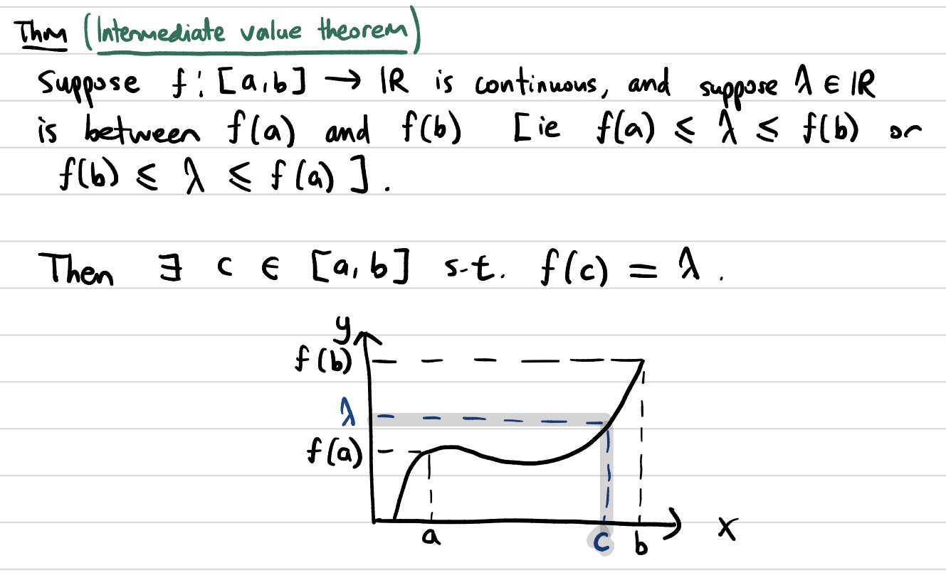
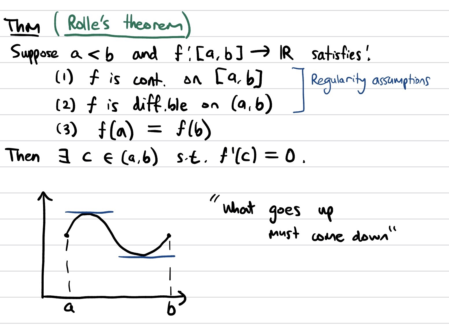
- Differentiation. This chapter formalises what a derivative means, and proves several related theorems like the linear approximation theorem, Rolle’s Theorem, and the Mean Value Theorem.
I really enjoyed solving the problem sets for this module. The definitions and theorems often feel quite mysterious at first glance, but through some deep thought during problem solving, you really see why these definitions and theorems make sense and get some intuitive pictures of what they mean. Ultimately, I felt quite a deep appreciation for the mechanics of maths, seeing so many big ideas developed from such unassuming axioms.
I don’t think my enjoyment of this module is shared by the majority though. Apparently, a couple hundred people scored less than 50% on the Jan midsessional exams (which are essentially mock exams). Many find the learning curve for this module in particular to be EXTREMELY steep, due to the proof-based nature of Analysis that is unlike anything seen at high school.
Advice for those taking this module:
- Learn the definitions and theorems precisely, including all the regularity assumptions (i.e. the assumptions that just ensure your mathematical object is “well behaved” enough). For example, for Rolle’s Theorem or the Mean Value Theorem, you should always state that the function \(f\) is continuous on \([a, b]\) and differentiable on \((a, b)\).
- Think deeply about the subtleties - what breaks if you drop a certain assumption/why are certain assumptions needed in the first place? Continuing with the Rolle’s Theorem/Mean Value Theorem example: why do we have to assume that \(f\) is continuous on \([a, b]\) AND differentiable on \((a, b)\) when another result in the module says that differentiability implies continuity?2
- Learn all the tools at your disposal and a general idea of when you should apply them. For example, when proving that an infinite series converges, there are seven different tests you can apply. You should have several examples of series you can apply these tests to.
- Collect a list of counterexamples. When you learn a new theorem, it is incredibly helpful to know examples of functions or sequences where the theorem fails because one condition isn’t met. For example, a classic example of a continuous function that is not differentiable on \(\mathbb{R}\) is \(f(x) = |x|\). An example of an unbounded continuous function on \((0, \infty)\) is \(f(x) = 1/x\).
- Be prepared for anything. The lecturer has set fairly, routine easy exams in the past but decided to step up the difficulty significantly in May 2026, and set a paper that I thought genuinely tested deep understanding.
MATH0004 Analysis 2
This module is a natural follow-up to Analysis 1, with the objective of developing a rigourous theory of integration, and then some. Again, I think this is another fantastic module, so I am putting this straight into S tier.
A rough breakdown what the module covers:
- Cauchy sequences and uniform continuity. On its own, not a very interesting chapter, and is intended just as a warmup. However, Cauchy sequences in particular, sequences that get “really close” to each other as they progress, turn out to be very important in further mathematics. Formally:
A sequence \(x_n\) is Cauchy if for every \(\varepsilon > 0\), there exists \(N \in \mathbb{N}\) such that for all \(m, n > N\), \(|x_m - x_n| < \varepsilon\).
Riemann Integration. From the ground up, instead of loosely understanding integration as “area under the curve”, the Riemann integral is formally defined using Upper and Lower Darboux sums. We see a proof of the Fundamental Theorem of Calculus, a theorem used a ton at high school without much justification for why it works.
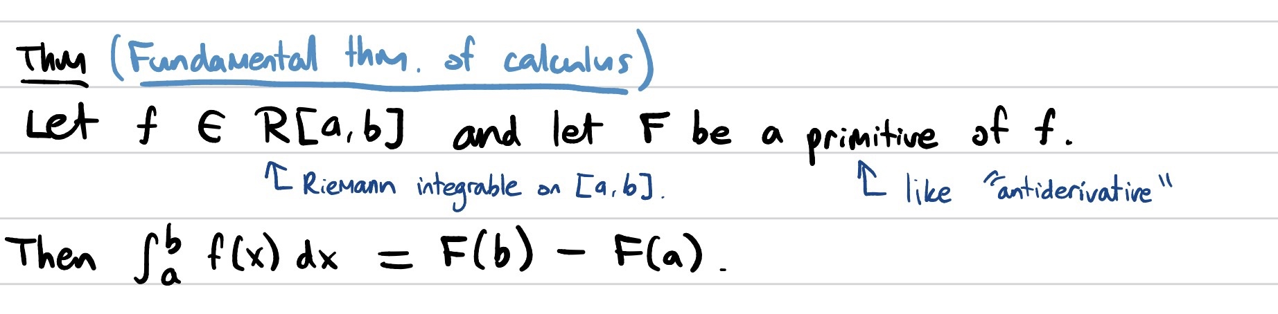
Figure: Fundamental Theorem of Calculus
Proofs are also given for other fundamental tools like integration by parts and integration by substitution, which is cool.Power series. We investigate the properties of infinite series of the form \(\sum_{n=0}^{\infty} a_n x^n\), where \(a_n\) are coefficients and \(x \in \mathbb{R}\) is an independent variable. The main goal of this chapter is proving that you can differentiate and integrate them term-by-term under certain conditions. Power series are seen quite a lot in maths, for example, in Maclaurin/Taylor series. One great application of the theorems proven here is analytically justifying why \(\frac{d}{dx} exp(x) = exp(x)\) and \(\frac{d}{dx} \sin(x) = \cos(x)\).
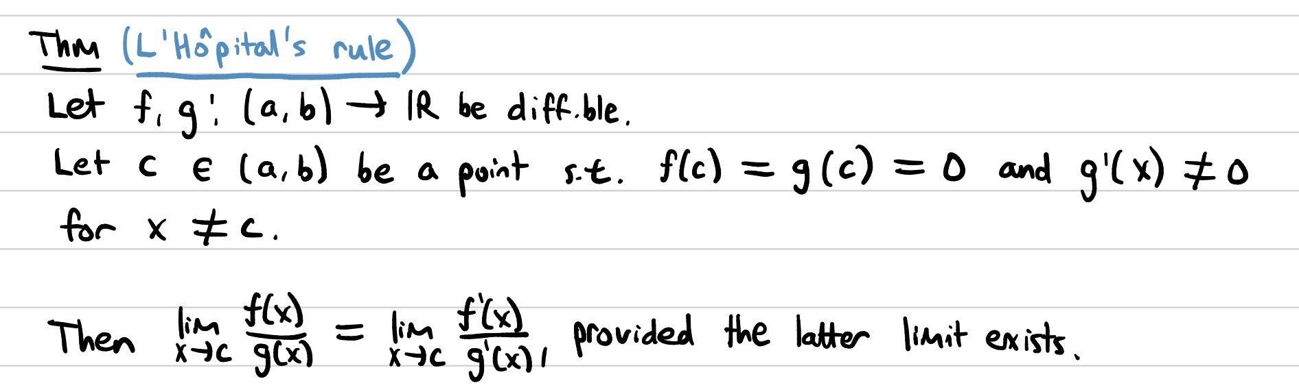
L’Hôpital’s rule and Taylor’s theorem (which is a more general version of Maclaurin’s theorem). We prove these two theorems encountered at A-level, which is neat.
- Improper integrals. An improper integral is, loosely speaking, an integral where something “goes wrong” - either the interval of integration is infinite, or the function blows up somewhere in the interval. This chapter is about how to prove they converge. Some examples:
Overall, I really enjoyed this module, gaining a really deep intuition of all the things informally examined at A-level.
Advice and thoughts for those taking this module (on top of the advice given for Analysis 1):
- The heaviest module of first year. The lecturer has said this is the module with the lowest averages across all first-year modules.
- The lecturer has kindly made typed lecture notes available (unlike the Analysis 1 lecturer), which is a great refernece to check exactly what is and isn’t examinable.
- The lecturer has also made all past papers since 1997 available, which is amazing. The syllabus has not changed in the last 15 or so years, and the lecturer for this module has not changed since I was born3 so the exam style is fairly consistent.
- In some sense, this is the easiest module to score 100% on, as 1. there is so much “bookwork” (reciting definitions, theorem statements, and proofs covered in lectures) on this exam and 2. there are barely any new questions, they are all recycled from prior years. Do the past papers!
- When learning the lemmas/theorems for this module, I found that it is often the case that the proof kind of obscures the statement and is (counterintuitively) unhelpful for understanding why the lemma/theorem is true in the first place. For example, the proof for the Taylor theorem and L’Hopital (in my opinion) does not help you understand why they are true, as they rely on some gimmicky tricks. To that end…
- When learning the lemmas/theorems for this module, I found it helpful to immediately find exam questions where they can be applied, which is helpful for understanding the statement itself.
- Don’t gamble on proofs. The sheer number of proofs in this module makes it tempting to skip learning a few of them (and some really took me a long time to nail down). But they are the easiest marks to get and a tragedy to lose. Some proofs in this module can be worth so many marks. For example, the proof for Cauchy’s General Principle of Convergence was worth 17 marks on one particular exam.
MATH0005 Algebra 1
Work in progress.
Draft. This course is an introduction to linear algebra, extending the basic matrix and vector concepts introduced in A-Level. I think this module is the one I have the hardest time explaining it in intuitive terms to those without a Mathematics background, as the ideas feel very abstract.
I HATE ROW REDUCTION.
MATH0006 Algebra 2
Work in progress.
Draft. An introduction to abstract algebra, the study of algebraic structures, the study of symmetry. The module is about zooming out and looking at the underlying structure of many mathematical operations and how they’re really the same under a certain lens. Another fantastic module imo, S tier.
The main topics:
- Basic number theory and permutations. Primes, divisors, Euclid’s algorithm (an efficient way to compute the GCD of two integers), modular arithmetic. Just a warmup to the course, nothing too exciting.
Further thoughts on the module:
- Everyone’s favourite lecturer out of the Year 1 lecturers, props to Ed Segal.
- Best exam performance of mine here, scored 98/100 on this one. The lecturer is a really generous exam setter, could have set a really really diffcult exam given the nature of the module.
MATH0008 Applied Mathematics
This module is about modelling some real world phenomena. There are two distinct chunks to this module. The first half is about modelling population dynamics using difference and differential equations. The second half is about classical mechanicals: forces, oscillations, collisions, and the wave equation.
Some highlights:
- Population dynamics. We looked at how populations grow, die off, and sometimes compete. One model we looked at was the Lotka–Volterra equations
, which models predator-prey dynamics (think foxes and rabbits). Another model we looked at was the SIR model
(Susceptible, Infective, Removed), which is a model of how disease spreads through a population. They can be visualised with “phase planes”. For example, the figure below shows how a predator (y) and prey (x) interact.
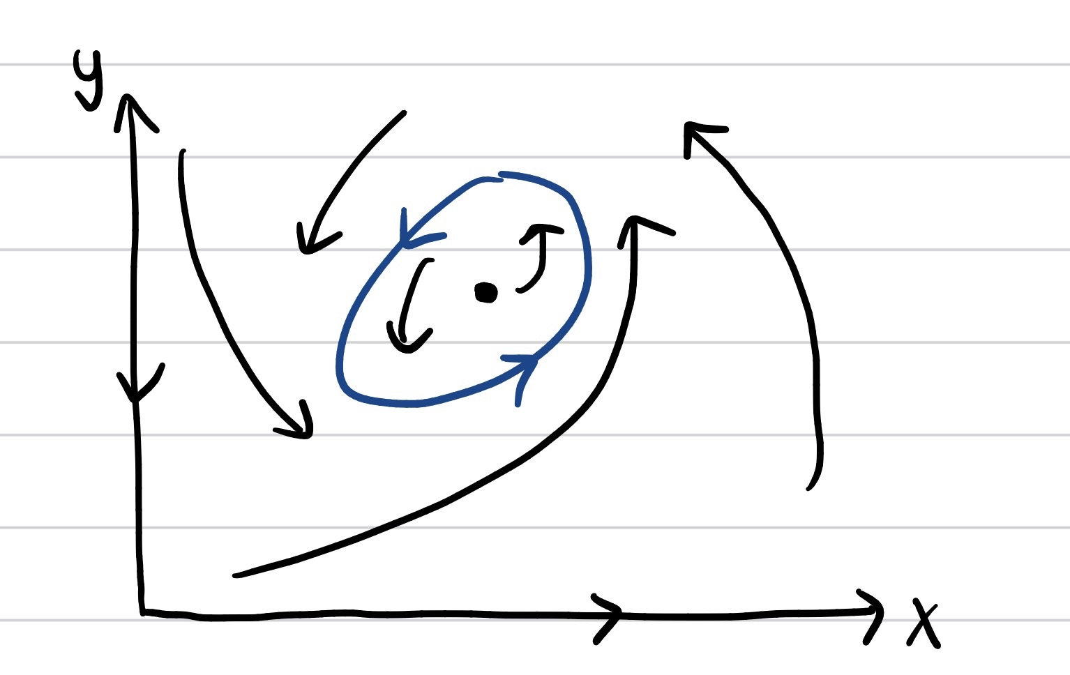
Figure: Phase plane for a predator-prey system.
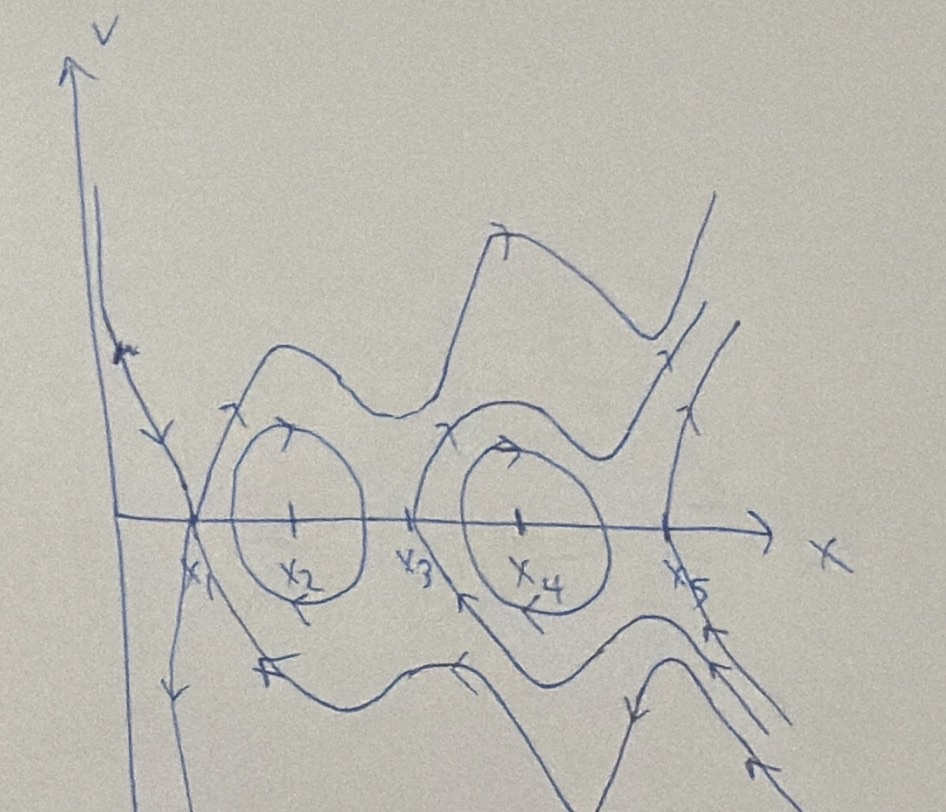
Phase planes aren’t just seen in the biology section of the course thouhgh, they can also be applied to mechanics problems.
- The wave equation. I was incredibly confused when learning about this topic in lectures for the first time, though it did eventually click. We saw the derivation of the so-called wave equation, which describes how waves (like sound, light, or water ripples) move through space and time:\(\frac{\partial^2 u}{\partial t^2} = c^2 \frac{\partial^2 u}{\partial x^2}\)which solves to:\(u(x,t) = \sum_{n=1}^{\infty} \sin\left(\frac{n\pi x}{L}\right)\left[C_n \cos\left(\frac{n\pi ct}{L}\right) + D_n \sin\left(\frac{n\pi ct}{L}\right)\right]\)
The solution to this equation is very interesting! It says that when a string is plucked, its motion is actually infinitely many simple sine waves all superposed on top of each other, each oscillating at its own frequency \(\frac{n\pi c}{L}\), and each weighted by coefficients \(C_n\) and \(D_n\) that depend entirely on how you initially plucked the string. So what you hear from a plucked guitar string is really the result of many frequencies stacked together.
Overall, I liked the module content, and thought it tackled a variety of interesting problems. You also get to draw some cool diagrams! It’s going in B tier for me.
Advice/further thoughts for those taking the module:
- My main gripe with this module: the lecturer sets absolutely brutal exams. The median for the Jan midsessional was a low 45%, and about 40% of people that sat the exam failed it. I don’t have access to the data for the final May exam, but it was harder than the Jan exam for sure, and my coursemates mostly agreed that Applied was one of their worst (if not worst) exam out of all the May exams. Personally, I scored 68% on the final exam, which was a good 20% lower than my scores in all other modules.
- The lecturer likes to include high-mark items, with frequent 10 markers and 15 markers. In the May exam, it was very annoying that a 10 marker depended on getting the previous 15 marker correct, which led to me dropping a bunch of marks at once since I couldn’t get the 15 marker. Point being - make sure your algebra is strong and that you are highly confident in applying the methods in the course without making calculation errors early on.
MATH0009 Newtonian Mechanics
This module is about particle dynamics, extending ideas developed in A-level mechanics into 3D space. Two key themes in this module: first, developing useful coordinate systems (such as intrinsic coordinates, plane polar coordinates, and cylindrical polar coordinates), and second, using vector calculus and solving differential equations.
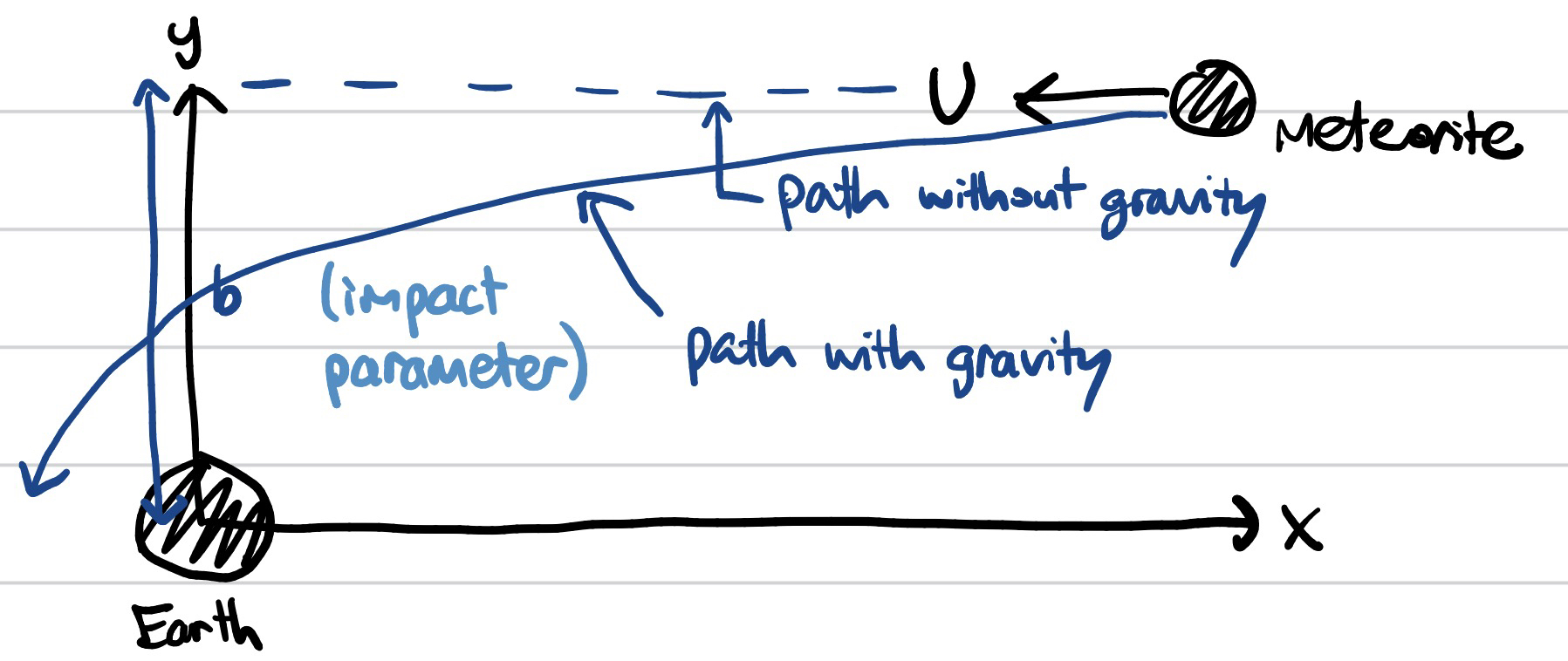
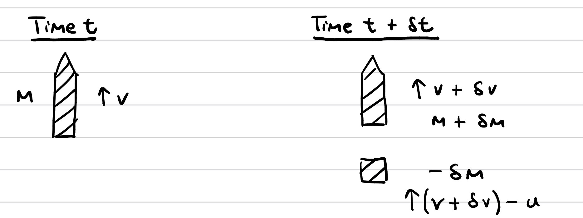
Like with MATH0008 Applied Maths, here are quite a few interesting problems and ideas tackled in the course. Highlights include using intrinsic coordinates to model the motion of particles sliding on a wire, calculating the trajectory of meteorites, and exploring rocket propulsion by analysing systems with variable mass.
I liked this module enough, so I’ll place it in B tier. I personally found that learning about the coordinate systems was kind of dull, and the problem-solving tended to rely on too many unmotivated algebraic tricks rather than physical intuition.
Advice for those taking the module:
- Check if your solutions make sense physically.
- There are a lot of formulas in this module that you want to ensure you can derive quickly.
- When in doubt, dot with the velocity vector \(\dot{r}\).
MATH0010 Mathematical Methods 1
A module that aims to bring everyone coming from a range of different syllabi up to speed on a range of basic topics: vectors, complex numbers, univariate and multivariate calculus, and differential equations.
There isn’t that much to this module imo. It’s well delivered and does its job of easing everyone into university mathematics, but it’s not really deeply interesting, so I’ll put it in C tier.
Here are the topics. Most are already seen in A-level Further Maths so I won’t elaborate much.
- Vectors. Scalar and vector products, equations of lines and planes, and one of the most challenging topics in the course: Einstein summation notation. It’s a way of writing vector expressions that can sometimes be more useful. For example, the cross product can be rewritten as \((\mathbf{a} \times \mathbf{b})_i = \epsilon_{ijk} a_j b_k\).
- Complex numbers.
- Basic differentiation and integration.
- Multivariable calculus.
- Differential equations.
- Basic probability theory, which is kind of randomly tacked on to the end of the course.
Advice for those taking the module:
- Don’t be intimidated by the Einstein summation notation. Even if you don’t completely understand what it is, just learn the identities. All you have to do is apply them mechanically in the exam.
- Despite the module content being (relatively) easy, don’t underestimate the exam, the lecturer has set some exams that I found quite tough relative to other modules.
- Make sure you’re familiar with all the content in the module, especially the nicher parts like t-sub, improper integrals.
- It’s not worthwhile to spend the time to do the computation for every single past exam question for both Methods 1 and 2. They take such a long time and don’t really aid understanding either. Just make sure you know how to set up the methods.
MATH0011 Mathematical Methods 2
This module is split into two distinct halves.
The first half is introductory Python, assuming no prior programming knowledge. It covers Python fundamentals: data types, functions and scope, conditionals, loops, and object-oriented programming. I love programming, but since it’s completely introductory, I found it rather dull. I am really looking forward to taking some computational mathematics modules in year 2/3 though like Computational Methods, Numerical Methods, and Combinatorial Optimisation.
The second half continues the study of multivariable calculus. Some topics include:
- Double and triple integrals. These are useful for calculating multidimensional properties like area, volume, mass, and center of mass. They look like:
Vector fields and operations. Three essential vector operations: \(\nabla f\), \(\nabla \cdot \mathbf{F}\), \(\nabla \times \mathbf{F}\). They apparently show up everywhere in Physics, like in Maxwell’s equations, fluid dynamics, and the Schrödinger equation.
Surface integrals. Calculating the surface area of three dimensional objects. Two big theorems of calculus introduced here: Stokes’ theorem and the Gauss Divergence theorem.
\(\oint_{\partial S} \mathbf{F} \cdot d\mathbf{r} = \iint_S (\nabla \times \mathbf{F}) \cdot d\mathbf{S}\) \(\oiint_{\partial V} \mathbf{F} \cdot d\mathbf{S} = \iiint_V (\nabla \cdot \mathbf{F}) \, dV\)
They look intimidating (and they are, I still don’t fully understand what they do yet and I know there’s more of this next year :/ ), but can be viewed as higher dimensional extensions of the Fundamental Theorem of Calculus (discussed in the MATH0004 Analysis 2 section). They relate an integral over a boundary to an integral over the region inside.
There are some interesting concepts here and there, but overall I didn’t really enjoy the module that much. It did not answer any questions I found particularly interesting. Also, answering coursework and exam questions for this module was for the most part, annoying, as the computations are really really long. Like Methods 1, although for different reasons, I’ll put this one in C tier.
Further thoughts/advice for those taking the module:I don’t think I fully understood the module by the end of it, but I was good at looking at a question and knowing exactly what kind of computation I was being asked to do. Even though the module is conceptually harder than Methods 1, most exam questions just ask you to perform long computations without having to think about anything too deeply, so it is definitely relatively easier to score higher marks on this module.